Data processing with MIMA
How to use MIMA to process your shotgun metagenomics data.
This section shows you how to use the MIMA pipeline for data processing of shotgun metagenomics sequenced reads using the assembly-free approach.
MIMA: data-processing
This section covers the data processing pipeline, which consists of three main modules:
| Module | |
|---|
| Quality control (QC) of the sequenced reads | 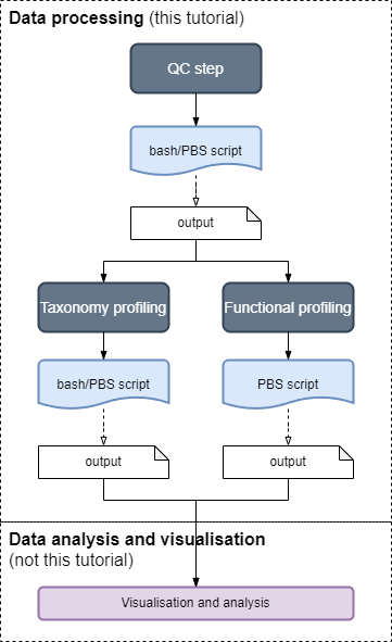 |
| Taxonomy profiling after QC, for assigning reads to taxon (this step can be run in parallel with step 3) |
| Functional profiling after QC, for assigning reads to genes (this step can be run in parallel with step 2) |
Note
The
Analysis and Visualisation comes after the data has been processed and is covered in the
analysis tutorialsHow the tutorials works
The tutorials are split into the three modules:
Each module has six sub-sections where actions are required in steps 2 to 6.
- A brief introduction
- RUN command to generate PBS scripts
- Check the generated PBS scripts
- RUN command to submit PBS scripts as jobs
- Check the expected outputs after PBS job completes
- RUN Post-processing step (optional steps are marked)
Check list
For this set of tutorials, you need
- Access to High-performance cluster (HPC) with a job scheduling system like OpenPBS
- HPC system must have
Apptainer or Singularity installed
- Install MIMA Container image
- start an interactive PBS job
- create the image sandbox
- set the
SANDBOX environment variable
- Take note of the paths for the reference databases, namely
- MiniMap2 host reference genome file
- Kraken2 and Bracken reference database (same directory for the two tools)
- HUMAnN reference databases
- MetaPhlAn reference databases
- Understand the need to know points
- Data processing worked on paired-end sequenced reads with two files per sample
- forward read fastQ files usually has some variation of _R1.fq.gz or _1.fq.gz filename suffix, and
- reverse read fastQ files usually some variation of _R2.fq.gz or _1.fq.gz filename suffix
- Download tutorial data and check the manifest file
1 - Download tutorial data
metadata and sequence data files for shotgun metagenomics data-processing
In the data processing tutorials, we will use data from the study by
Tourlousse, et al. (2022), Characterization and Demonstration of Mock Communities as Control Reagents for Accurate Human Microbiome Community Measures, Microbiology Spectrum.
This data set consists of two mock communities: DNA-mock and Cell-mock. The mock communities consists of bacteria that are mainly detected the human gastrointestinal tract ecosystem with a small mixture of some skin microbiota. The data was processed in three different labs: A, B and C. In the previous tutorial, , we only processed a subset of the samples (n=9). In this tutorial we will be working with the full data set which has been pre-processed using the same pipeline. In total there were 56 samples of which 4 samples fell below the abundance threshold and therefore the final taxonomy abundance table has 52 samples. We will train the random forest classifier to distinguish between the three labs.
- The raw reads are available from NCBI SRA Project PRJNA747117, and there are 56 paired-end samples (112 fastq files)
- As the data is very big we will work with a subset (n=9 samples, 18 fastq files)
- This tutorial teaches you how to prepare the required raw fastq files
Note
You will need about 80GB of disk space depending on which option you used for downloading.
Step 1) Download tutorial files
wget https://github.com/mrcbioinfo/mima-pipeline/raw/master/examples/mima_tutorial.zip
- Extract the archived file using
unzip
- Check the directory structure matches using
tree
~/mima_tutorial
├── ftp_download_files.sh
├── manifest.csv
├── pbs_header_func.cfg
├── pbs_header_qc.cfg
├── pbs_header_taxa.cfg
├── raw_data
└── SRA_files
Note! Assumed working directory
This tutorial assumes the
~/mima_tutorial directory is located in your
home directory as indicated by the
~ (tilde) sign. If you have put the files in another location then replace all occurrences of
~/mima_tutorial with your location (remember to use
absolute paths).
Data files
| File | Description |
|---|
| ftp_download_files.sh | direct download FTP links used in Option A: direct download below |
| SRA_files | contains the SRA identifier of the 9 samples used in Option B and Option C below |
| manifest.csv | comma separated file of 3 columns, that lists the sampleID, forward_filename, reverse_filename |
| pbs_header_*.cfg | PBS configuration files that contain specific parameters for job submissions |
Step 2) Download Sequence files
Choose from the 3 options for downloading the tutorial data depending on your environment setup:
| Option | Tool | Est. size | Description |
|---|
| A | curl | 24GB | direct download using curl command, files are already compressed |
| B | sratoolkit
(installed on system) | 75GB | download using sratoolkit which is available on your system or via modules The files are not compressed when downloaded; compression is a post-processing step |
| C | sratoolkit
(installed in MIMA) | 75GB | installed in MIMA container; same as option B downloaded files are not compressed |
Option A: direct download
- Run the following command for direct download
bash FTP_download_files.sh
- Download the SRA files using
prefetch command
prefetch --option-file SRA_files --output-directory raw_data
Below is the output, wait until all files are downloaded
2022-09-08T05:50:42 prefetch.3.0.0: Current preference is set to retrieve SRA Normalized Format files with full base quality scores.
2022-09-08T05:50:42 prefetch.3.0.0: 1) Downloading 'SRR17380209'...
2022-09-08T05:50:42 prefetch.3.0.0: SRA Normalized Format file is being retrieved, if this is different from your preference, it may be due to current file availability.
2022-09-08T05:50:42 prefetch.3.0.0:  Downloading via HTTPS...
...
- After download finish, check the downloaded files with the
tree command
raw_data/
├── SRR17380115
│   └── SRR17380115.sra
├── SRR17380118
│   └── SRR17380118.sra
├── SRR17380122
│   └── SRR17380122.sra
├── SRR17380209
│   └── SRR17380209.sra
├── SRR17380218
│   └── SRR17380218.sra
├── SRR17380222
│   └── SRR17380222.sra
├── SRR17380231
│   └── SRR17380231.sra
├── SRR17380232
│   └── SRR17380232.sra
└── SRR17380236
    └── SRR17380236.sra
- Extract the fastq files using the
fasterq-dump command - We’ll also save some disk space by zipping up the fastq files using
bzip (or pigz)
cd ~/mima_tutorial/raw_data
fasterq-dump --split-files */*.
bzip2 *.fastq
tree .
.
├── SRR17380115
│   └── SRR17380115.sra
├── SRR17380115_1.fastq.gz
├── SRR17380115_2.fastq.gz
├── SRR17380118
│   └── SRR17380118.sra
├── SRR17380118_1.fastq.gz
├── SRR17380118_2.fastq.gz
├── SRR17380122
│   └── SRR17380122.sra
├── SRR17380122_1.fastq.gz
├── SRR17380122_2.fastq.gz
├── SRR17380209
│   └── SRR17380209.sra
├── SRR17380209_1.fastq.gz
├── SRR17380209_2.fastq.gz
├── SRR17380218
│   └── SRR17380218.sra
├── SRR17380218_1.fastq.gz
├── SRR17380218_2.fastq.gz
├── SRR17380222
│   └── SRR17380222.sra
├── SRR17380222_1.fastq.gz
├── SRR17380222_2.fastq.gz
├── SRR17380231
│   └── SRR17380231.sra
├── SRR17380231_1.fastq.gz
├── SRR17380231_2.fastq.gz
├── SRR17380232
│   └── SRR17380232.sra
├── SRR17380232_1.fastq.gz
├── SRR17380232_2.fastq.gz
├── SRR17380236
│   └── SRR17380236.sra
├── SRR17380236_1.fastq.gz
└── SRR17380236_2.fastq.gz
Option C: download via MIMA
- This options assumes you have installed MIMA and set up the
SANDBOX environment variable - Download the SRA files using the following command
apptainer exec $SANDBOX prefetch --option-file SRA_files --output-directory raw_data
- Below is the output, wait until all files are downloaded
2022-09-08T05:50:42 prefetch.3.0.0: Current preference is set to retrieve SRA Normalized Format files with full base quality scores.
2022-09-08T05:50:42 prefetch.3.0.0: 1) Downloading 'SRR17380209'...
2022-09-08T05:50:42 prefetch.3.0.0: SRA Normalized Format file is being retrieved, if this is different from your preference, it may be due to current file availability.
2022-09-08T05:50:42 prefetch.3.0.0:  Downloading via HTTPS...
...
- After download finishes, check the downloaded files
raw_data/
├── SRR17380115
│   └── SRR17380115.sra
├── SRR17380118
│   └── SRR17380118.sra
├── SRR17380122
│   └── SRR17380122.sra
├── SRR17380209
│   └── SRR17380209.sra
├── SRR17380218
│   └── SRR17380218.sra
├── SRR17380222
│   └── SRR17380222.sra
├── SRR17380231
│   └── SRR17380231.sra
├── SRR17380232
│   └── SRR17380232.sra
└── SRR17380236
    └── SRR17380236.sra
- Extract the fastq files using the
fasterq-dump command - We’ll also save some disk space by zipping up the fastq files using
bzip (or pigz)
cd ~/mima_tutorial/raw_data
singularity exec $SANDBOX fasterq-dump --split-files */*.
singularity exec $SANDBOX bzip2 *.fastq
tree .
.
├── SRR17380115
│   └── SRR17380115.sra
├── SRR17380115_1.fastq.gz
├── SRR17380115_2.fastq.gz
├── SRR17380118
│   └── SRR17380118.sra
├── SRR17380118_1.fastq.gz
├── SRR17380118_2.fastq.gz
├── SRR17380122
│   └── SRR17380122.sra
├── SRR17380122_1.fastq.gz
├── SRR17380122_2.fastq.gz
├── SRR17380209
│   └── SRR17380209.sra
├── SRR17380209_1.fastq.gz
├── SRR17380209_2.fastq.gz
├── SRR17380218
│   └── SRR17380218.sra
├── SRR17380218_1.fastq.gz
├── SRR17380218_2.fastq.gz
├── SRR17380222
│   └── SRR17380222.sra
├── SRR17380222_1.fastq.gz
├── SRR17380222_2.fastq.gz
├── SRR17380231
│   └── SRR17380231.sra
├── SRR17380231_1.fastq.gz
├── SRR17380231_2.fastq.gz
├── SRR17380232
│   └── SRR17380232.sra
├── SRR17380232_1.fastq.gz
├── SRR17380232_2.fastq.gz
├── SRR17380236
│   └── SRR17380236.sra
├── SRR17380236_1.fastq.gz
└── SRR17380236_2.fastq.gz
Step 3) Check manifest
- Examine the manifest file
cat mima_tutorial/manifest.csv
- Your output should looking like something below
- Check column 2 (
FileID_R1) and column 3 (FileID_R2) match the names of the files in raw_data
- Update the manifest file as required
Sample_ID,FileID_R1,FileID_R2
SRR17380209,SRR17380209_1.fastq.gz,SRR17380209_2.fastq.gz
SRR17380232,SRR17380232_1.fastq.gz,SRR17380232_2.fastq.gz
SRR17380236,SRR17380236_1.fastq.gz,SRR17380236_2.fastq.gz
SRR17380231,SRR17380231_1.fastq.gz,SRR17380231_2.fastq.gz
SRR17380218,SRR17380218_1.fastq.gz,SRR17380218_2.fastq.gz
SRR17380222,SRR17380222_1.fastq.gz,SRR17380222_2.fastq.gz
SRR17380118,SRR17380118_1.fastq.gz,SRR17380118_2.fastq.gz
SRR17380115,SRR17380115_1.fastq.gz,SRR17380115_2.fastq.gz
SRR17380122,SRR17380122_1.fastq.gz,SRR17380122_2.fastq.gz
Manifest file formats
- the first row is the header and is case sensitive, it must have the three columns:
Sample_ID,FileID_R1,FileID_R2 - the filenames in columns 2 and 3 do not need to be absolute paths as the directory where the files are located will be specified during quality checking
Remember to check out what else you need to know before jumping into quality checking
2 - Need to know
preparation for data-processing tutorials
Project working directory
After downloading the tutorial data, we assume that the mima_tutorial is the working directory located in your home directory (specified by the tilde, ~). Hence, we will try to always make sure we are in the right directory first before executing a command, for example, run the following commands:
$ cd ~/mima_tutorial
$ tree .
- the starting directory structure for
mima_tutorial should look something like:
mima_tutorial
├── ftp_download_files.sh
├── manifest.csv
├── pbs_header_func.cfg
├── pbs_header_qc.cfg
├── pbs_header_taxa.cfg
├── raw_data/
    ├── SRR17380115_1.fastq.gz
    ├── SRR17380115_2.fastq.gz
    ├── ...
...
From here on, ~/mima_tutorial will refer to the project directory as depicted above. Replace this path if you saved the tutorial data in another location.
TIP: Text editors
There are several places where you may need to edit the commands, scripts or files. You can use the vim text editors to edit text files directly on the terminal.
For example, the command below lets you edit the pbs_head_qc.cfg text file
Containers and binding paths
When deploying images, make sure you check if you need to bind any paths.
PBS configuration files
The three modules (QC, Taxonomy profiling and Function profiling) in the data-processing pipeline require access to a job queue and instructions about the resources required for the job. For example, the number of CPUs, the RAM size, the time required for execution etc. These parameters are defined in PBS configuration text files.
Three such configuration files are in provided after you have downloaded the tutorial data. There are 3 configuration files, one for each module as they require different PBS settings indicated by lines starting with the #PBS tags.
 1
 2
 3
 4
 5
 6
 7
 8
 9
10
11
| #!/bin/bash
#PBS -N mima-qc
#PBS -l ncpus=8
#PBS -l walltime=2:00:00
#PBS -l mem=64GB
#PBS -j oe
set -x
IMAGE_DIR=~/mima-pipeline
export APPTAINER_BIND="</path/to/source1>:</path/to/destination1>,</path/to/source2>:</path/to/destination2>"
|
PBS settings | Description |
|---|
#PBS -N | name of the job |
#PBS -l ncpus | number of CPUs required |
#PBS -l walltime | how long the job will take, here it’s 2 hours. Note check the log files whether your jobs have completed correctly or failed due to not enough time |
#PBS -l mem=64GB | how much RAM the job needs, here it’s 64GB |
#PBS -l -j oe | standard output logs and error logs are concatenated into one file |
Use absolute paths
When running the pipeline it is best to use full paths when specifying the locations of input files, output files and reference data to avoid any ambiguity.
Absolute/Full paths
always start with the root directory, indicated by the forward slash (/) on Unix based systems.
- e.g., below changes directory (
cd) to a folder named scripts that is located in the user jsmith’s home directory. Provided this folder exists, then this command will work from anywhere on the filesystem."
[~/metadata] $ cd /home/jsmith/scripts
Relative paths
are relative to the current working directory
- Now imagine the following file system structure in the user
john_doe’s home directory - The asterisks marks his current location, which is inside the
/home/user/john_doe/studyAB/metadata sub-folder
/home/user/john_doe
├── apps
├── reference_data
├── studyABC
│   ├── metadata **
│   ├── raw_reads
│   └── analysis
├── study_123
├── scripts
└── templates
- In this example we are currently in the
metadata directory, and change directory to a folder named data that is located in the parent directory (..) - This command only works provided there is a
data folder in the parent directory above metadata - According to the filesystem above, the parent directory of
metadata is studyABC and there is no data subfolder in this directory, so this command will fail with an error message
[/home/user/john_doe/studyABC/metadata] $ cd ../data
-bash: cd: ../data: No such file or directory
Now that you have installed the data and know the basics, you can begin data processing with quality control.
3 - Quality control (QC)
QC module in MIMA, check reads are of high standard
This step must be done before Taxonomy and Function profiling.
Introduction: QC module
Quality control (QC) checks the sequenced reads obtained from the sequencing machine is of good quality. Bad quality reads or artefacts due to sequencing error if not removed can lead to spurious results and affect downstream analyses. There are a number of tools available for checking the read quality of high-throughput sequencing data.
This pipeline uses the following tools:
Workflow description
One bash (*.sh) script per sample is generated by this module that performs the following steps. The module also generates $N$ number of PBS scripts (set using the --num-pbs-jobs parameter).
This tutorial has 9 samples spread across 3 PBS jobs. One PBS job will execute three bash scripts, one per sample.
| Step | |
|---|
| 1. repair.sh from BBTools/BBMap tool suite, repairs the sequenced reads and separates out any singleton reads (orphaned reads that are missing either the forward or reverse partner read) into its own text file. |  |
| 2. dereplication using clumpify.sh from BBTools/BBMap tool suite, removes duplicate reads and clusters reads for faster downstream processing |
| 3. quality checking is done with fastp.sh and checks the quality of the reads and removes any reads that are of low quality, too long or too short |
| 4. decontamination with minimap2.sh maps the sequenced reads against a reference genome (e.g., human) defined by the user. It removes these host-reads from the data and generates a cleaned output file. This becomes the input for taxonomy profiling and function profiling modules. |
| The (optional) last step generates a QC report text file with summary statistics for each file. This step is run after all PBS scripts have been executed for all samples in the study. |
For details about the tool versions, you can check the MIMA container image installed
Step 1. Generate QC PBS scripts
- Tick off the check list
- Find the absolute path to the host reference genome file (e.g., Human host might use GRCh38_latest_genome.fna)
- Replace the highlighted line
--ref <path/to/human/GRCh38_latest_genome.fna> to the location of your host reference genome file - Enter the following command
- the backslash (
\) at the end of each line informs the terminal that the command has not finished and there’s more to come (we broke up the command for readability purposes to explain each parameter below) - note if you enter the command as one line, remove the backslashes
1
2
3
4
5
6
7
8
| apptainer run --app mima-qc $SANDBOX \
-i ~/mima_tutorial/raw_data \
-o ~/mima_tutorial/output \
-m ~/mima_tutorial/manifest.csv \
--num-pbs-jobs 3 \
--ref <path/to/human/GRCh38_latest_genome.fna> \
--mode container \
--pbs-config ~/mima_tutorial/pbs_header_qc.cfg
|
Parameters explained
Parameter | Required? | Description |
|---|
-i <input> | yes | must be absolute path to the directory where fastq files are stored. FastQ files often have the *.fastq.gz or *.fq.gz extension. This path is used to find the FileID_R1 and FileID_R2 columns specified in the manifest.csv file |
-o <output> | yes | absolute path output directory where results will be saved. The <output> path will be created if it does not exists. Note if there are already existing subdirectories in the <output> path, then this step will fail. |
-m <manifest.csv> | yes | a comma-separated file (*.csv) that has three columns with the headers: Sample_ID, FileID_R1, FileID_R2 see the example below. Note the fileID_R1 and fileID_R2 are relative to the -i <input> path provided. |
--num-pbs-jobs | no
(default=4) | number of PBS scripts to generate by default 4 jobs are created with samples split equally between the jobs |
--ref | yes | path to the host genome file GRCh38_latest_genome.fna |
--mode container | no
(default=‘single’) | set this if you are running as a Container |
--pbs-config | yes if
--mode container | path to the pbs configuration file, must specify this parameter if --mode container is set |
tip
These commands can get really long, you can use Notepad to
- copy & paste the commands
- change the paths and parameters as desired
- copy & paste to the terminal
Or you can explore using the vim text editor.
Step 2. Check generated scripts
- After step 1, you should see the new directory:
~/mima_tutorial/output - Inside
output/, there should be a sub-directory QC_module - Inside
output/QC_module, there should be 3 PBS scripts with the *.pbs file extension
- only the
output folder is shown in the snapshot below
~/mima_tutorial
└── output/
    └──  QC_module
      ├── CleanReads
      ├── qcModule_0.pbs
      ├── qcModule_1.pbs
      ├── qcModule_2.pbs
      ├── QCReport
      ├── SRR17380115.sh
      ├── SRR17380118.sh
      ├── SRR17380122.sh
      ├── SRR17380209.sh
      ├── SRR17380218.sh
      ├── SRR17380222.sh
      ├── SRR17380231.sh
      ├── SRR17380232.sh
      └── SRR17380236.sh
Step 3. Submit QC jobs
- Let’s examine one of the PBS scripts to be submitted
cat ~/mima_tutorial/output/QC_module/qcModule_0.pbs
- Your PBS script should look something like below, with some differences
- line 10:
IMAGE_DIR should be where you installed MIMA and build the sandbox - line 11:
APPTAINER_BIND should be setup during installation when binding paths- make sure to include the path where the host reference genome file is located
- line 14:
/home/user is replaced with the absolute path to your actual home directory
 1
 2
 3
 4
 5
 6
 7
 8
 9
10
11
12
13
14
15
16
17
18
| #!/bin/bash
#PBS -N QC_module_0
#PBS -l ncpus=8
#PBS -l walltime=2:00:00
#PBS -l mem=64GB
#PBS -j oe
set -x
IMAGE_DIR=~/mima-pipeline
export APPTAINER_BIND="/path/to/human/GRCh38:/path/to/human/GRCh38"
cd /home/user/mima_tutorial/output/QC_module/
apptainer exec ${IMAGE_DIR} bash /home/user/mima_tutorial/output/QC_module/SRR17380209.sh > SRR17380209_qc_module.log 2>&1
apptainer exec ${IMAGE_DIR} bash /home/user/mima_tutorial/output/QC_module/SRR17380232.sh > SRR17380232_qc_module.log 2>&1
apptainer exec ${IMAGE_DIR} bash /home/user/mima_tutorial/output/QC_module/SRR17380236.sh > SRR17380236_qc_module.log 2>&1
|
- Navigate to the
~/mima_tutorial/output/QC_module - Submit the PBS job using
qsub
cd ~/mima_tutorial/output/QC_module
qsub qcModule_0.pbs
- You can check the job has been submitted and their status with
qstat - Repeat the
qsub command for each of the qcModule_1.pbs and qcModule_2.pbs files - Wait until all PBS jobs have completed
PBS log files
- Usually a PBS job will generate a log file in the same directory from where the job was submitted
- As such we changed directory to where the PBS scripts are saved to submit the jobs because the log files are required for the Step 5. Generating the QC report.
Step 4. Check QC outputs
- After all PBS job completes, you should have the following outputs
tree ~/mima_tutorial/output/QC_module
- We only show outputs for one sample below with
... meaning “and others” - You’ll have a set of output files for each sample listed in the
manifest.csv (provided the corresponding *.fastq files exists)
 ~/mima_tutorial/output/QC_module
├── CleanReads
│   ├── SRR17380209_clean_1.fq.gz
│   ├── SRR17380209_clean_2.fq.gz
│   └── ...
├── QC_module_0.o3492023
├── qcModule_0.pbs
├── qcModule_1.pbs
├── qcModule_2.pbs
├── QCReport
│   ├── SRR17380209.json
│   ├── SRR17380209.outreport.html
│   └── ...
├── ...
├── SRR17380209_qc_module.log
├── SRR17380209.sh
├── SRR17380209_singletons.fq.gz
└── ...
Step 5. (optional) Generate QC report
- You can generate a summary QC Report after all samples have been quality checked
- This step can be run directly from the command line
- First navigate to the
QC_module directory that have the qc_module.log files
cd ~/mima_tutorial/output/QC_module
apptainer run --app mima-qc-report $SANDBOX \
-i ~/mima_tutorial/output/QC_module \
--manifest ~/mima_tutorial/manifest.csv
Troubleshoot
If your sequence read files are not saved in your home directory, check you have set up the APPTAINER_BIND environment variable when
binding paths.
The output is a comma separated text file located in ~/mima_tutorial/output/QC_module/QC_report.csv.
- Examine the output report using
headcolumn formats the text file as columns like a table for readabilty
head ~/mima_tutorial/output/QC_module/QC_report.csv | column -t -s ','
- Your output should resemble something like below
- the numbers can be different due to different tool versions
- The
log_status column specify if log files were found, other values mean- missing QC log: missing *qc_module.log file for the corresponding sample
- missing JSON log: missing fastp *.json file for the corresponding sample
SampleId     log_status      Rawreads_seqs  Derep_seqs  dedup_percentage  Post_QC_seqs  low_quality_reads(%)  Host_seqs  Host(%)                 Clean_reads
SRR17380209  OK              14072002       14045392.0  0.0809091         9568710       31.87295876113675     426.0      0.004452010772611982    9568284.0
SRR17380232  OK              11822934       11713130.0  0.0706387         11102358      5.214421764293575     62.0       0.0005584399278063273   11102296.0
SRR17380236  OK              11756456       11656800.0  0.0688868         10846582      6.950603939331549     46.0       0.00042409673388354047  10846536.0
SRR17380231  OK              12223354       12104874.0  0.069757          11414164      5.7060486544510916    14.0       0.00012265462455244203  11414150.0
SRR17380218  OK              14913690       14874174.0  0.0856518         11505850      22.645452446636703    234.0      0.002033748049905048    11505616.0
SRR17380222  OK              16927002       16905928.0  0.0980011         11692516      30.83777477344042     294.0      0.002514428887674817    11692222.0
SRR17380118  OK              40393998       40186880.0  0.234584          40148912      0.09447859599949038   100242.0   0.2496755080187478      40048670.0
Next: you can now proceed with either Taxonomy Profiling with MIMA or Function Profiling with MIMA.
4 - Taxonomy Profiling
assign reads to taxa, generating a taxonomy feature table ready for analysis
Introduction to Taxonomy Profiling
Taxonomy profiling takes the quality controlled (clean) sequenced reads as input and matches them against a reference database of previously characterised sequences for taxonomy classification.
There are many different classification tools, for example: Kraken2, MetaPhlAn, Clark, Centrifuge, MEGAN, and many more.
This pipeline uses Kraken2 and Bracken abundance estimation. Both require access to reference database or you can generate your own reference data. In this pipeline, we will use the GTDB database (release 95) and have built a Kraken2 database.
Workflow description
Kraken2 requires big memory (~300GB) to run, so there is only one PBS script that will execute each sample sequentially.
In this tutorial, we have 9 samples which will be executed within one PBS job.
Steps in the taxonomy profiling module:
| Step | |
|---|
| Kraken2 assigns each read to a lowest common ancestor by matching the sequenced reads against a reference database of previously classified species |  |
| Bracken takes the Kraken2 output to estimate abundances for a given taxonomic rank. This is repeated from Phylum to Species rank. |
| Generate feature table is performed after all samples assigned to a taxa and abundances estimated. This step combines the output for all samples and generates a feature table for a given taxonomic rank. The feature table contains discrete counts and relative abundances of "taxon X occurring in sample Y". |
Step 1. Generate PBS script
Before starting, have you understood the need to know points?
- After QC checking your sequence samples and generating a set of
CleanReads - Find the absolute paths for the Kraken2 and Bracken reference databases on your HPC system (!! they need to be in the same directory)
- Replace the highlighted line
--reference-path <path/to/Kraken2_db> with the Kraken2 absolute path- the backslash (
\) at the end of each line informs the terminal that the command has not finished and there’s more to come (we broke up the command for readability purposes to explain each parameter below) - note if you enter the command as one line, remove the backslashes
1
2
3
4
5
6
7
8
| apptainer run --app mima-taxa-profiling $SANDBOX \
-i ~/mima_tutorial/output/QC_module/CleanReads \
-o ~/mima_tutorial/output \
--reference-path </path/to/Kraken2_db> \
--read-length 150 \
--threshold 100 \
--mode container \
--pbs-config ~/mima_tutorial/pbs_header_taxa.cfg
|
Parameters explained
Parameter | Required? | Description |
|---|
-i <input> | yes | full path to the ~/mima_tutorial/output/QC_module/CleanReads directory that was generated from Step 1) QC, above. This directory should hold all the *_clean.fastq files |
-o <output> | yes | full path to the ~/mima_tutorial/output directory where you would like the output files to be saved, can be the same as Step 1) QC |
--reference-path | yes | full path to the reference database (this pipeline uses the GTDB release 95 reference database) |
--read-length | no (default=150) | read length for Bracken estimation, choose the value closest to your sequenced read length (choose from 50, 75, 100 and 150) |
--threshold | no (default=1000) | Bracken filtering threshold, features with counts below this value are filtered in the abundance estimation |
--mode container | no (default=single) | set this if you are running as a Container. By default, the PBS scripts generated are for the ‘standalone’ option, that is without Singularity |
--pbs-config | yes if --mode container | path to the pbs configuration file (see below). You must specify this parameter if --mode container is set. You do not need to set this parameter if running outside of Singularity |
If you changed the file extension of the cleaned files or are working with already cleaned files from somewhere else, you can specify the forward and reverse suffix using:
Parameter | Required? | Description |
|---|
--fwd-suffix | default=_clean_1.fq.gz | file suffix for cleaned forward reads from QC module |
--rev-suffix | default=_clean_2.fq.gz | file suffix for cleaned reverse reads from QC module |
Step 2. Check generated scripts
- After Step 1, you should see in the output directory:
~/mima_tutorial/output/Taxonomy_profiling- one PBS script
- one bash script/sample (total of 9 bash scripts in this tutorial)
- Have a look at the directory structure using
tree
tree ~/mima_tutorial/output/Taxonomy_profiling
Expected directory structure
- bracken/ and kraken2/ are subdirectories created by Step 2 to store the output files after PBS job is executed
.
├── bracken
├── featureTables
│   └── generate_bracken_feature_table.py
├── kraken2
├── run_taxa_profiling.pbs
├── SRR17380209.sh
├── SRR17380232.sh
├── SRR17380236.sh
└── ...
Step 3. Submit Taxonomy job
- Let’s examine the PBS script to be submitted
cat ~/mima_tutorial/output/Taxonomy_profiling/run_taxa_profiling.pbs
- Your PBS script should look something like below, with some differences
- line 10:
IMAGE_DIR should be where you installed MIMA and build the sandbox - line 11:
APPTAINER_BIND should be setup during installation when binding paths- make sure to include the path where the host reference genome file is located
- line 14:
/home/user is replaced with the absolute path to your actual home directory
 1
 2
 3
 4
 5
 6
 7
 8
 9
10
11
12
13
14
15
16
17
18
| #!/bin/bash
#PBS -N mima-taxa
#PBS -l ncpus=28
#PBS -l walltime=10:00:00
#PBS -l mem=300GB
#PBS -j oe
set -x
IMAGE_DIR=~/mima-pipeline
export APPTAINER_BIND="/path/to/kraken2/reference_database:/path/to/kraken2/reference_database"
cd /home/user/mima_tutorial/output/Taxonomy_profiling/
apptainer exec ${IMAGE_DIR} bash /home/user/mima_tutorial/output/Taxonomy_profiling/SRR17380209.sh
apptainer exec ${IMAGE_DIR} bash /home/user/mima_tutorial/output/Taxonomy_profiling/SRR17380232.sh
...
|
Tip: when running your own study
- increase the wall-time if you have a lot of samples
- increase the memory as needed
- Change directory to
~/mima_tutorial/output/Taxonomy_profiling - Submit PBS job using
qsub
cd ~/mima_tutorial/output/Taxonomy_profiling
qsub run_taxa_profiling.pbs
- You can check the job statuses with
qstat - Wait for the job to complete
Step 4. Check Taxonomy outputs
- After the PBS job completes, you should have the following outputs
tree ~/mima_tutorial/output/Taxonomy_profiling
- Only a subset of the outputs are shown below with
... meaning “and others” - You’ll have a set of output for each sample that passed the QC step
~/mima_tutorial/output/Taxonomy_profiling
├── bracken
│   ├── SRR17380218_class
│   ├── SRR17380218_family
│   ├── SRR17380218_genus
│   ├── SRR17380218.kraken2_bracken_classes.report
│   ├── SRR17380218.kraken2_bracken_families.report
│   ├── SRR17380218.kraken2_bracken_genuses.report
│   ├── SRR17380218.kraken2_bracken_orders.report
│   ├── SRR17380218.kraken2_bracken_phylums.report
│   ├── SRR17380218.kraken2_bracken_species.report
│   ├── SRR17380218_order
│   ├── SRR17380218_phylum
│   ├── SRR17380218_species
│   └── ...
├── featureTables
│   └── generate_bracken_feature_table.py
├── kraken2
│   ├── SRR17380218.kraken2.output
│   ├── SRR17380218.kraken2.report
│   ├── ...
│   ├── SRR17380231.kraken2.output
│   └── SRR17380231.kraken2.report
├── QC_module_0.o3492470
├── run_taxa_profiling.pbs
├── SRR17380209.sh
├── SRR17380218_bracken.log
├── SRR17380218.sh
├── SRR17380222_bracken.log
├── SRR17380222.sh
├── SRR17380231_bracken.log
├── SRR17380231.sh
├── SRR17380232.sh
└── SRR17380236.sh
Output files
| Directory / Files | Description |
|---|
| output | specified in the --output-dir <output> parameter set in step 1b) |
| Taxonomy_profiling | contains all files and output from this step |
| Taxonomy_profiling/*.sh | are all the bash scripts generated by step 2b) for taxonomy profiling |
| Taxonomy_profiling/run_taxa_profiling.pbs | is the PBS wrapper generated by step 2b) that will execute each sample sequentially |
| Taxonomy_profiling/bracken | consists of the abundance estimation files from Bracken, one per sample, output after PBS submission |
| Taxonomy_profiling/featureTables | consists of the merged abundance tables generated by step 2e) below |
| Taxonomy_profiling/kraken2 | consists of the output from Kraken2 (two files per sample), output after PBS submission |
See the tool website for further details about the Kraken2 output and Bracken output
Step 5. Generate taxonomy abundance table
- After all samples have been taxonomically annotated by Kraken2 and abundance estimated by Bracken, we need to combine the tables
- Navigate to
~/mima_tutorial/output/Taxonomy_profiling/featureTables - Run the commands below directly from terminal (not a PBS job)
- Check the output with
tree
cd ~/mima_tutorial/output/Taxonomy_profiling/featureTables
apptainer exec $SANDBOX python3 generate_bracken_feature_table.py
tree .
- All bracken output files will be concatenated into a table, one for each taxonomic rank from Phylum to Species
- table rows are taxonomy features
- table columns are abundances
- By default, the tables contain two columns for one sample: (i) discrete counts and (ii) relative abundances
- The
generate_bracken_feature_table.py will split the output into two files with the suffices:_counts for discrete counts and_relAbund for relative abundances
.
├── bracken_FT_class
├── bracken_FT_class_counts
├── bracken_FT_class_relAbund
├── bracken_FT_family
├── bracken_FT_family_counts
├── bracken_FT_family_relAbund
├── bracken_FT_genus
├── bracken_FT_genus_counts
├── bracken_FT_genus_relAbund
├── bracken_FT_order
├── bracken_FT_order_counts
├── bracken_FT_order_relAbund
├── bracken_FT_phylum
├── bracken_FT_phylum_counts
├── bracken_FT_phylum_relAbund
├── bracken_FT_species
├── bracken_FT_species_counts
├── bracken_FT_species_relAbund
├── combine_bracken_class.log
├── combine_bracken_family.log
├── combine_bracken_genus.log
├── combine_bracken_order.log
├── combine_bracken_phylum.log
├── combine_bracken_species.log
└── generate_bracken_feature_table.py
Step 6. (optional) Generate summary report
- You can generate a summary report after the Bracken abundance estimation step
- This step can be run directly from the command line
- You need to specify the absolute input path (
-i parameter)- this is the directory that contains the
*_bracken.log files, by default these should be in the output/Taxonomy_profiling directory - update this path if you have the
*_bracken.log files in another location
apptainer run --app mima-bracken-report $SANDBOX \
-i ~/mima_tutorial/output/Taxonomy_profiling
- The output is a tab separated text file
- By default, the output file
bracken-summary.tsv will be in the same location as the input directory. You can override this using the -o parameter to specify the full path to the output file. - Examine the output report using
headcolumn formats the text file as columns like a table for readability
head ~/mima_tutorial/output/Taxonomy_profiling/bracken-summary.tsv | column -t
- Your output should resemble something like below (only the first 9 columns are shown in the example below)
- numbers might be different depending on the threshold setting or tool version
sampleID     taxon_rank  log_status             threshold  num_taxon  num_tx_above_thres  num_tx_below_thres  total_reads  reads_above_thres
SRR17380209  phylum      ok-reads_unclassified  100        96         21                  75                  4784142      4449148
SRR17380209  class       ok-reads_unclassified  100        230        21                  209                 4784142      4438812
SRR17380209  order       ok-reads_unclassified  100        524        53                  471                 4784142      4404574
SRR17380209  family      ok-reads_unclassified  100        1087       103                 984                 4784142      4363888
SRR17380209  genus       ok-reads_unclassified  100        3260       228                 3032                4784142      4239221
SRR17380209  species     ok-reads_unclassified  100        8081       571                 7510                4784142      3795061
SRR17380232  phylum      ok-reads_unclassified  100        87         21                  66                  5551148      5216610
SRR17380232  class       ok-reads_unclassified  100        207        19                  188                 5551148      5201532
SRR17380232  order       ok-reads_unclassified  100        464        51                  413                 5551148      5165978
SRR17380232  family      ok-reads_unclassified  100        949        105                 844                 5551148      5126854
Next: if you haven’t already, you can also generate functional profiles with your shotgun metagenomics data.
5 - Functional Profiling
assign reads to gene families and pathways, generating a function feature table ready for analysis
Introduction to Functional Profiling
Functional profiling, like taxonomy profiling, takes the cleaned sequenced reads after QC checking as input and matches them against a reference database of previously characterised gene sequences.
There are different types of functional classification tools available. This pipeline uses the HUMAnN3 pipeline, which also comes with its own reference databases.
Workflow description
One PBS script per sample is generated by this module. In this tutorial, we have 9 samples, so there will be 9 PBS scripts.
Steps in the functional profiling module:
| Steps | |
|---|
HUMAnN3 is used for processing and generates three outputs for each sample:
- gene families
- pathway abundances
- pathway coverage
|  |
| Generate feature table is performed after all samples have been processed. This combines the output and generates a feature table that contains the abundance of gene/pathway X in sample Y. |
Step 1. Generate PBS scripts
Before starting, have you understood the need to know points?
- After QC checking your sequence samples and generating a set of
CleanReads - Find the absolute paths for the HUMAnN3 and MetaPhlAn reference databases depending on the MIMA version you installed
- Replace the highlighted lines with the absolute path for the reference databases
path/to/humann3/chocophlanpath/to/humann3/unirefpath/to/humann3/utility_mappingpath/to/metaphlan_databases
- the backslash (
\) at the end of each line informs the terminal that the command has not finished and there’s more to come (we broke up the command for readability purposes to explain each parameter below) - note if you enter the command as one line, remove the backslashes
1
2
3
4
5
6
7
8
9
| apptainer run --app mima-function-profiling $SANDBOX \
-i ~/mima_tutorial/output/QC_module/CleanReads \
-o ~/mima_tutorial/output \
--nucleotide-database </path/to>/humann3/chocophlan \
--protein-database /<path/to>/humann3/uniref \
--utility-database /<path/to>/humann3/utility_mapping \
--metaphlan-options "++bowtie2db /<path/to>/metaphlan_databases" \
--mode container \
--pbs-config ~/mima_tutorial/pbs_header_func.cfg
|
Parameters explained
Parameter | Required? | Description |
|---|
-i <input> | yes | full path to the ~/mima_tutorial/output/QC_module/CleanReads directory that was generated from Step 1) QC, above. This directory should hold all the *_clean.fastq files |
-o <output> | yes | full path to the ~/mima_tutorial/output output directory where you would like the output files to be saved, can be the same as Step 1) QC |
--nucleotide-database <path> | yes | directory containing the nucleotide database, (default=/refdb/humann/chocophlan) |
--protein-database <path> | yes | directory containing the protein database, (default=/refdb/humann/uniref) |
--utility-database <path> | yes | directory containing the protein database, (default=/refdb/humann/utility_mapping) |
--metaphlan-options <string> | yes | additional MetaPhlAn settings, like specifying the bowtie2 reference database (default="++bowtie2db /refdb/humann/metaphlan_databases"). Enclose parameters in double quotes and use ++ for parameter settings. |
--mode container | no (default=‘single’) | set this if you are running in the Container mode |
--pbs-config | yes if --mode container | path to the pbs configuration file (see below). You must specify this parameter if --mode container is set. You do not need to set this parameter if running outside of Singularity |
--mpa3 | no | this parameter is only applicable for MIMA container with MetaPhlAn4. You can set --mpa3 for backward compatibility with MetaPhlAn3 databases |
Step 2. Check PBS scripts output
- After step 1, you should see in the output directory:
~/mima_tutorial/output/Function_profiling
tree ~/mima_tutorial/output/Function_profiling
- There should be one PBS script/sample (total of 9 bash scripts in this tutorial)
...
├── featureTables
│   ├── generate_func_feature_tables.pbs
│   └── generate_func_feature_tables.sh
├── SRR17380209.pbs
├── SRR17380218.pbs
├── SRR17380222.pbs
├── SRR17380231.pbs
├── SRR17380232.pbs
└── SRR17380236.pbs
Step 3. Submit Function jobs
- Let’s examine one of the PBS scripts
$ cat ~/mima_tutorial/output/Function_profiling/SRR17380209.pbs
- Your PBS script should look something like below, with some differences
- line 10:
IMAGE_DIR should be where you installed MIMA and build the sandbox - line 11:
APPTAINER_BIND should be setup during installation when binding paths- make sure to include the path where the host reference genome file is located
- line 14:
/home/user is replaced with the absolute path to your actual home directory - lines 22-25: ensure the paths to the reference databases are all replaced (the example below uses the vJan21 database version and the parameter
index is sent to MetaPhlAn to disable autocheck of index) - note that the walltime is set to 8 hours
 1
 2
 3
 4
 5
 6
 7
 8
 9
10
11
12
13
14
15
16
17
18
19
20
21
22
23
24
25
26
| #!/bin/bash
#PBS -N mima-func
#PBS -l ncpus=8
#PBS -l walltime=8:00:00
#PBS -l mem=64GB
#PBS -j oe
set -x
IMAGE_DIR=~/mima-pipeline
export APPTAINER_BIND="/path/to/humann3_database:/path/to/humann3_database,/path/to/metaphlan_databases:/path/to/metaphlan_databases"
cd /home/user/mima_tutorial/output/Function_profiling/
# Execute HUMAnN3
cat /home/user/mima_tutorial/output/QC_module/CleanReads/SRR17380209_clean_1.fq.gz ~/mima_tutorial/output/QC_module/CleanReads/SRR17380209_clean_2.fq.gz > ~/mima_tutorial/output/Function_profiling/SRR17380209_combine.fq.gz
outdir=/home/user/mima_tutorial/output/Function_profiling/
apptainer exec ${IMAGE_DIR} humann -i ${outdir}SRR17380209_combine.fq.gz --threads 28 \
-o $outdir --memory-use maximum \
--nucleotide-database </path/to/humann3>/chocophlan \
--protein-database </path/to/humann3>/uniref \
--utility-database </path/to/humann3>/utility_mapping \
--metaphlan-options \"++bowtie2db /path/to/metaphlan_databases ++index mpa_vJan21_CHOCOPhlAnSGB_202103\" \
--search-mode uniref90
|
Tip: when running your own study
- increase the walltime if you have alot of samples
- increase the memory as needed
- Change directory to
~/mima_tutorial/output/Functional_profiling - Submit PBS job using
qsub
$ cd ~/mima_tutorial/output/Functional_profiling
$ qsub SRR17380209.pbs
- Repeat this for each
*.pbs file - You can check your job statuses using
qstat - Wait until all PBS jobs have completed
Step 4. Check Function outputs
- After all PBS jobs have completed, you should have the following outputs
$ ls -1 ~/mima_tutorial/output/Function_profiling
- Only a subset of the outputs are shown below with
... meaning “and others” - Each sample that passed QC, will have a set of functional outputs
featureTables
...
SRR17380115_combine_genefamilies.tsv
SRR17380115_combine_humann_temp
SRR17380115_combine_pathabundance.tsv
SRR17380115_combine_pathcoverage.tsv
SRR17380115.pbs
SRR17380118_combine_genefamilies.tsv
SRR17380118_combine_humann_temp
SRR17380118_combine_pathabundance.tsv
SRR17380118_combine_pathcoverage.tsv
SRR17380118.pbs
...
SRR17380236.pbs
Step 5. Generate Function feature tables
- After all samples have been functionally annotated, we need to combine the tables together and normalise the abundances
- Navigate to
~/mima_tutorial/output/Fuctional_profiling/featureTables - Submit the PBS script file
generate_func_feature_tables.pbs
$ cd <PROJECT_PATH>/output/Functional_profiling/featureTables
$ qsub generate_func_feature_tables.pbs
- Check the output
- Once the job completes you should have 7 output files beginning with the
merge_humann3table_ prefix
~/mima_tutorial/
└── output/
    ├── Function_profiling
    │   ├── featureTables
    │   ├── func_table.o2807928
    │   ├── generate_func_feature_tables.pbs
    │   ├── generate_func_feature_tables.sh
    │   ├── merge_humann3table_genefamilies.cmp_uniref90_KO.txt
    │   ├── merge_humann3table_genefamilies.cpm.txt
    │   ├── merge_humann3table_genefamilies.txt
    │   ├── merge_humann3table_pathabundance.cmp.txt
    │   ├── merge_humann3table_pathabundance.txt
    │   ├── merge_humann3table_pathcoverage.cmp.txt
    │   └── merge_humann3table_pathcoverage.txt
    ├── ...
Tip: if you want different pathway mappings
In the file generate_func_feature_tables.sh, the last step in the humann_regroup_table command uses the KEGG orthology mapping file, that is the -c parameter:
-g uniref90_rxn -c <path/to/>map_ko_uniref90.txt.gz
If you prefer other mappings than change this line accordingly before running the PBS job using generate_func_feature_tables.pbs
Congratulations !
You have completed processing your shotgun metagenomics data and are now ready for further analyses
Analyses usually take in either the taxonomy feature tables or functional feature tables